Schrödinger 1D Equation Solver

Introduction

The goal of this project is to create an easily usable numerical solver for the 1D time independent Schrödinger equation which has the following form:

- \frac{ℏ ^{2}}{2 m} \frac{d ^{2} ψ}{d x ^{2}} + V (x) ψ = E ψ

The numerical solver will produce a list of quantized Energy values for any potential, $V (x)$ , function. Where the potential function represents the potential energy of the surroundings. The resulting $∣ ψ (x) ∣^{2}$ probability distributions are graphed along with the energy values. This can be used to gather intuition about the quantum-mechanical properties of small particles along with demonstrating phenomenon such as tunneling.

Instruction of Use

When first launched two graphs will be visible. To view this document the About button is pressed. To edit the potential function and the integration settings press Settings.

Settings

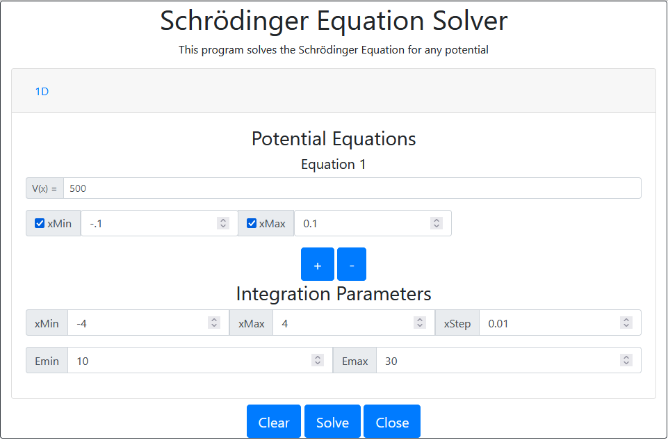
When settings is first opened the following menu will open.

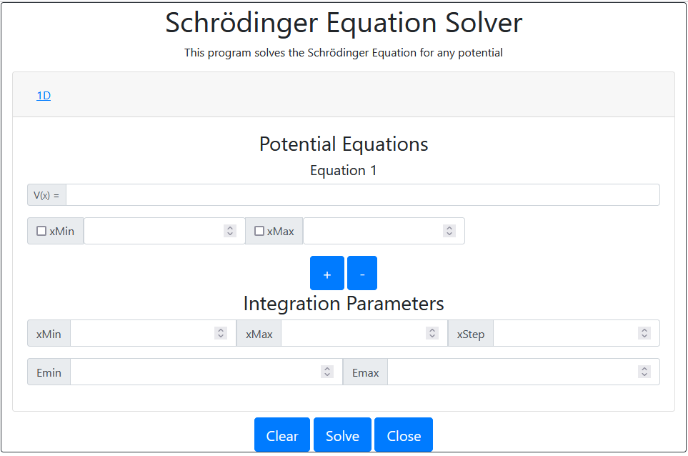
Currently only 1D graphing is supported.

Potential Equations

V(x) - enter a potential function in terms of x. Can use standard mathematical notation. Such as, sin, x^2, etc.
xMin - the lower bounds for the V(x) function specified. Check the box if the interval should be inclusive.
xMax- the upper bounds for theV(x) function specified. Check the box if the interval should be inclusive.

Functions can be added or removed using the "+" and "-".

Note: when adding or removing functions all the function data is cleared.

Note: the program assumes wave function only exists within the integration range. Thus it is important to keep this in mind and use potentials and integration ranges that sufficiently contain the wavefunction.

Integration Parameters

xMin - lower bounds for integration
xMax - upper bounds for integration
xStep - step size used in the numerical method
Emin - minimum energy value in search interval
Emax - maximum energy value in search interval

Note: Using a small step size and a large integration range can cause the webpage to become unresponsive.

Buttons

Clear - clears current graph data
Solve - runs numerical solver
Close - closes the setting menu returning to the graphs

Interpretation of Results

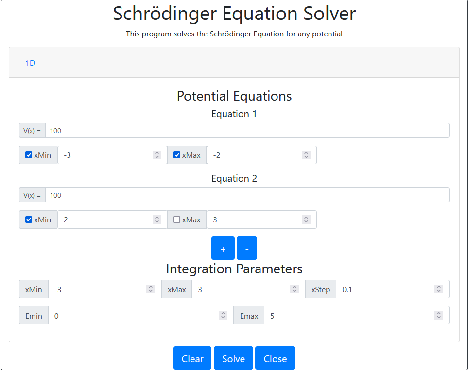
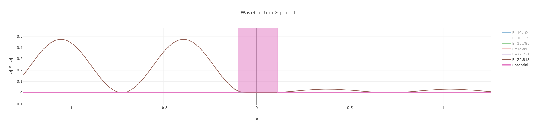
The following is a example function that approximates a infinite square well using a sufficiently large finite square well.

Settings

Results

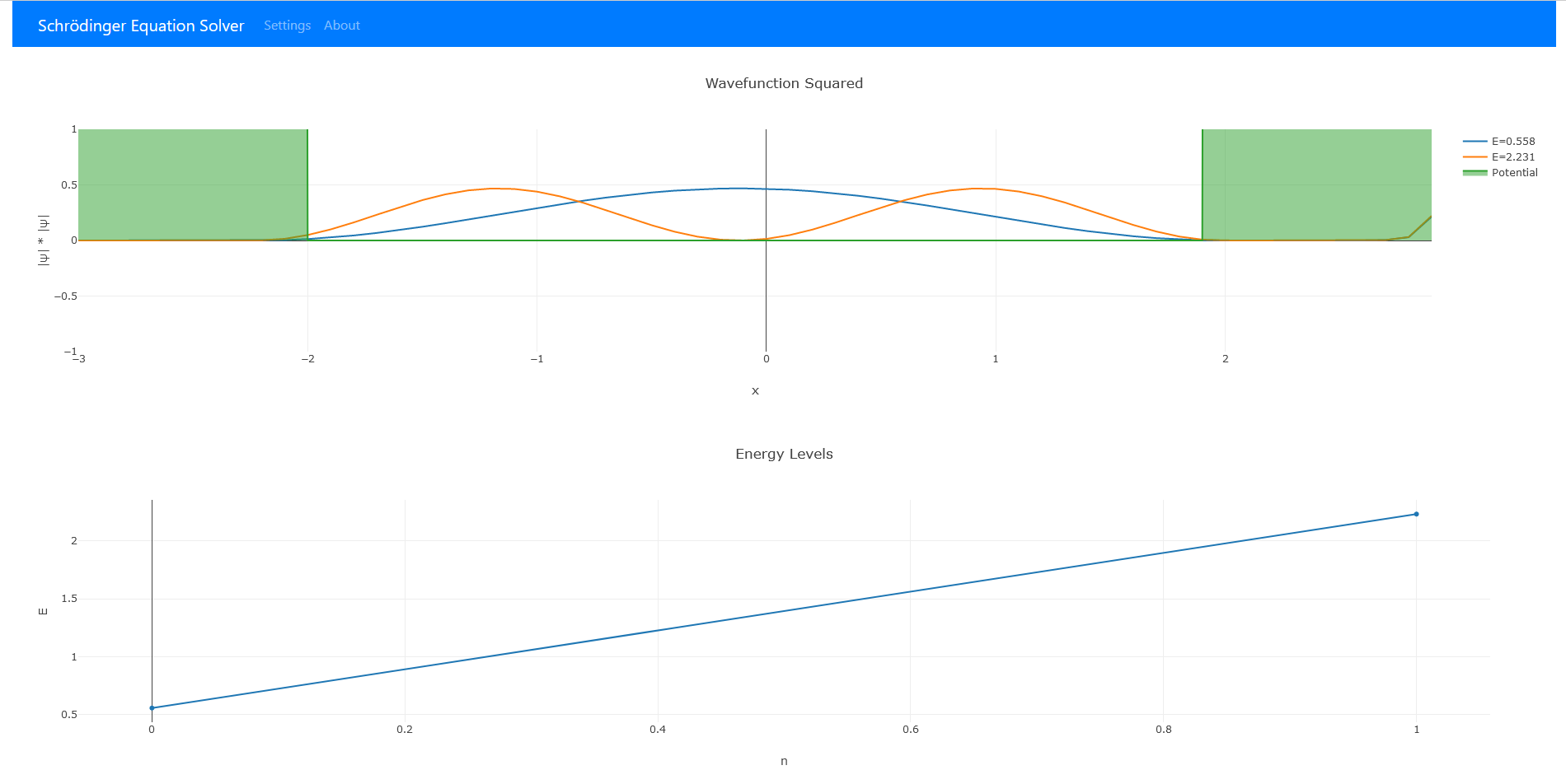
As can be seen two energy values were found between $(0, 5)$ . $E_{0} = 0.558$ and $E_{1} = 2.231$ . These two are then graphed in the top graph. The legend relates which is which and the shaded portions of the graph represent the potential function.

Both graphs can be interacted with by clicking and hovering will reveal accurate data information. In the upper right hand corner of both graphs there is also options to save each plot for future reference.

Following quantum mechanical principles the graphs can be interpreted according to the following equation.

P = \int_{a}^{b} ∣ ψ (x) ∣^{2} d x

In other words larger the area is under a specific energy graph the more likely it is to find a particle in that location. In addition, the energy trend in the lower graph can be used to predict a overall trend.

Methodology

This section will focus on the techniques used to numerical integrate the Schrödinger equation.

Initial Considerations

A few considerations were initially made to simplify the process. The main such consideration is that:

- \frac{ℏ ^{2}}{2 m} = c = - 1

This simplified calculations and does not alter the result beside with scaling. Additionally the solver is written to be able to assign $c$ to any value. However, this was omitted from the settings to increase simplicity.

Also to obtain definitive boundary conditions it is assumed the wavefunction only exists within the integration range.

Numerical Method

Many numerical methods could be used to solve the differential equation as it is only a second order. Despite the Numerov method being a common choice the 4th order Runge-Kutta method was chosen instead because if its increased flexibility.

Conversion Into a System of Equations

For use with the Runge-Kutta method the Schrödinger equation is converted into a system of differential equations. Carrying out the calculations and using:

z = \frac{d ψ}{d x}, \frac{d z}{d x} = \frac{d ^{2} ψ}{d x ^{2}}

yields:

z^{'} = \frac{y ( E - V ( x ) )}{c}

y^{'} = z

Now the Runge-Kutta method can be applied.

k_{1} l_{1} k_{2} l_{2} k_{3} l_{3} k_{4} l_{4} = f (x_{n}, y_{n}, z_{n}) Δ t = g (x_{n}, y_{n}, z_{n}) Δ t = f (x_{n} + \frac{Δ t}{2}, y_{n} + \frac{Δ k _{1}}{2}, z_{n} + \frac{Δ l _{1}}{2}) Δ x = g (x_{n} + \frac{Δ t}{2}, y_{n} + \frac{Δ k _{1}}{2}, z_{n} + \frac{Δ l _{1}}{2}) Δ x = f (x_{n} + \frac{Δ t}{2}, y_{n} + \frac{Δ k _{2}}{2}, z_{n} + \frac{Δ l _{2}}{2}) Δ x = g (x_{n} + \frac{Δ t}{2}, y_{n} + \frac{Δ k _{2}}{2}, z_{n} + \frac{Δ l _{2}}{2}) Δ x = f (x_{n} + Δ t, y_{n} + Δ k_{3}, z_{n} + Δ l_{3}) Δ x = g (x_{n} + Δ t, y_{n} + Δ k_{3}, z_{n} + Δ l_{3}) Δ x

Then to compute the next terms:

y_{n + 1} z_{n + 1} = y_{n} + \frac{k _{1} + 2 k _{2} + 2 k _{3} + k _{4}}{6} = z_{n} + \frac{l _{1} + 2 l _{2} + 2 l _{3} + l _{4}}{6}

Initial Value Considerations

Now that the numerical method is defined it is important to consider the initial values that must be used in the calculations.

Using the property the wave function:

1 = \int_{- \infty}^{\infty} ∣ ψ (x) ∣^{2} d x

Now since it was assumed the wavefunction only exits within the integration range the above equation can be modified.

1 = \int_{- x M i n}^{x M a x} ∣ ψ (x) ∣^{2} d x

This implies:

x \to x M i n + lim ψ (x) = x \to x M i n + lim \frac{d ψ ( x )}{d x} = 0

and similarly:

x \to x M a x - lim ψ (x) = x \to x M a x - lim \frac{d ψ ( x )}{d x} = 0

Now there are initial values and boundary conditions for both extremes of the integration range.

Conversion to a Boundary Condition Problem

Despite having initial conditions and boundary conditions for both extremes, Runge-Kutta only solves differential equations using starting initial conditions. To solve this a new function was defined.

f (E) = R u n g e K u t t a (E) ψ value at xMax

In other words given an energy level $E$ , $f (E)$ returns the value of $ψ$ at $x M a x$ . This is then used in conjunction with the bisection method to find the roots such that:

f (E) = 0

When a root is found it signified the energy value used satisfies the initial conditions and boundary conditions. Thus it is one of the quantized energy states.

Normalization

For each energy value the wavefunction is normalized according the following equation:

ψ_{n} (x) = \frac{ψ ( x )}{\int _{x M i n}^{x M a x} ∣ ψ ( x ) ∣ ^{2} d x}

However, a trapezoidal Reimann sum was used in place of the integration in the numerical calculations.

Validation

In order to validate the numerical accuracy the program was compared against known exact solutions.

Infinite Square Well

A infinite Square Well has an exact solution and can be approximated in the program as a finite square will with sufficient size. The exact solution is of the form:

E = \frac{( n + 1 ) ^{2} π ^{2}}{a ^{2}} = \frac{( n + 1 ) ^{2} π ^{2}}{1 0 0}

For a well with a length, $a$ of 5 units.

Program Settings

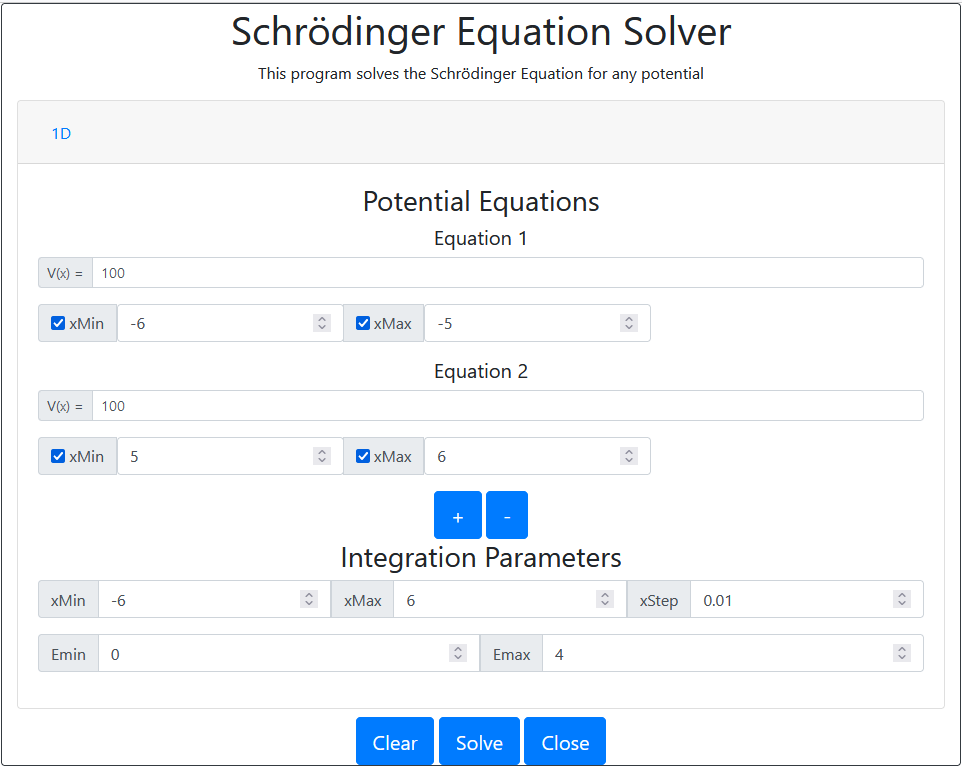
Results

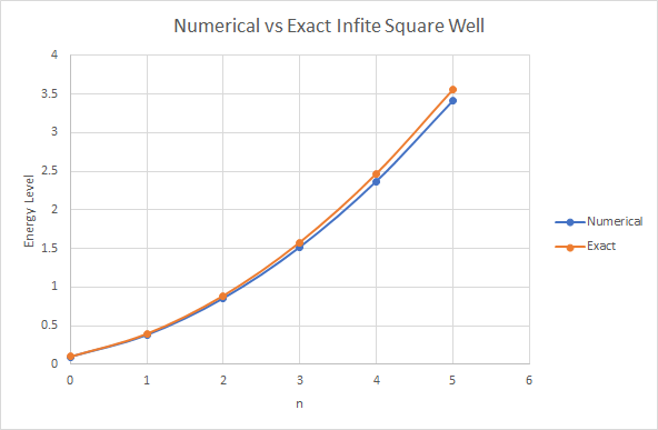
Energy Levels of Numerical vs Exact for Infinite Square Well

n	0	1	2	3	4	5
Numerical	0.095	0.379	0.854	1.518	2.371	3.414
Exact	0.099	0.394	0.888	1.579	2.467	3.55
Absolute Difference	0.004	0.016	0.034	0.061	0.096	0.139
Percent Difference	3.816%	4.080%	3.933%	3.948%	3.985%	3.992%

Conclusion

As can be seen above the numerical method is not exact but only has an error of about $4 %$ . The error can also be explained through approximating an infinite square wall with a large finite square wall. In either case the numerical solver is representative of the exact solution to a high degree of accuracy.

Tunneling

One of the most interesting applications of the program is to show a wavefunction that tunnels through a high barrier. For example take the following example:

Graph

As can be seen the waveform starts on the left side of the potential and tunnels through.